Convolutional Neural Network(CNN)

History of CNN

In 1963, Computer Scientist Larry Roberts, who is known as the father of computer vision described the possibility of extracting 3D geometrical information from 2D perspective views of blocks in his research called BLOCK WORLD. Many researchers worldwide in machine learning and artificial intelligence followed this work and studied computer vision in the context of BLOCK WORLD.

In this research, he said that it is important to understand simple edge-like shapes in images. He extracted these edge-like shapes from blocks to make the computer understand that these two blocks are the same irrespective of orientation.

In the 1970s, the first visual recognition algorithm, known as the generalized cylinder model, came from the AI lab at Stanford University. The idea here is that the world is composed of simple shapes and any real-world object is a combination of these simple shapes.

A Convolutional Neural Network is a Deep Learning algorithm that can take in an input image, assign importance (learnable weights and biases) to various aspects/objects in the image, and be able to differentiate one from the other.

It is composed of multiple building blocks, such as convolution layers, pooling layers, and fully connected layers, and is designed to automatically and adaptively learn hierarchies of features.

Applications of Convolution neural networks

1. Image Classification

IMAGE RECOGNITION

2. NLP

CNN models are effective for various NLP problems and achieved excellent results in sentence modeling, classification, and prediction.

3. OBJECT DETECTION

Style Transfer

Why do we use a Convolutional neural network over a Deep neural network?

Deep neural networks are prone to overfitting. Even slight changes in the training set cause the model a very different weight configuration.

Gradients can vanish in the long chain.

The terminology used in Convolutional neural network are:-

Kernel:-

The kernel is nothing but a filter that is used to extract the features from the images. The kernel is a matrix that moves over the input data, performs the dot product with the sub-region of input data, and gets the output as the matrix of dot products.

Activation function:-

The activation function decides whether a neuron should be activated or not by calculating the weighted sum and further adding bias with it. The purpose of the activation function is to introduce non-linearity into the output of a neuron.

output = Input x weight + bias

So we can see it’s in the form “y = MX + c”, So it’s in a straight line form, but to get more correct results, we need it to be curved, that’s when the activation function comes into the picture.

Some of the famous activation functions are:-

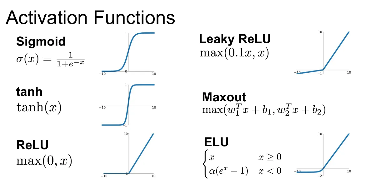
Convolutional layers:-

This layer is the first layer that is used to extract the various features from the input images. In this layer, the mathematical operation of convolution is performed between the input image and a filter of a particular size MxM. By sliding the filter over the input image, the dot product is taken between the filter and the parts of the input image concerning the size of the filter (MxM).

The convolution operation boils down to taking a given input and re-estimating it as a weighted average of all the inputs around it.

In 2D, we would consider neighbors along the rows and columns, using the following formula

K refers to kernel or weights and I refers to the input. And * refers to the convolution operation

Let a be the number of rows and b be the number of columns.m & n specify the size of the matrix.

Here is a pictorial representation using the above formulae.

Strides:-

Stride decides how our weight matrix should move in the input, i.e jumping one step or two.

In the example, we can see The weight matrix move in two places.

Padding:-

Padding is used when you don’t want to decrease the spatial resolution of the image when you use convolution.

Pooling:-

The pooling operation involves sliding a two-dimensional filter over each channel of the feature map and summarizing the features lying within the region covered by the filter.

Types of pooling are:-

1. Max pooling
2. Average pooling
3. Global pooling

MaxPooling layer:-We move a window across a feature map , where the maximum value within that window is the output.

Average pooling:- We move a window across a feature map , where the average value within that window is the output.

Global Pooling:- It is a pooling operation which generates one feature map for each corresponding category of the classification task in the last conv layer.

Learning rate:-

This is a parameter that decides how far the weights will move in the direction of the gradient. Intuitively it is like how quickly a network abandons old beliefs for new ones. If it is too small training will be slow, and If it is too large it may diverge.

DROPOUT:-

Dropout refers to dropping(not considering in both forward and backward pass) some neurons during the training phase. The neurons which are chosen at random.

We will make an image classifier using MNIST dataset with convolutional neural networks.

Dataset Info:-

1. 60,000 labeled digit images for training and 10,000 for testing.
2. Grayscale 28-by-28 pixel images(784 features) each represented by NumPy array.
3. Labels = 0 to 9

Basically, the Model will produce an array of 10 probabilities indicates that digits belong to which class (0 to 9).

Import all the library which are required to build the model.

Load dataset and some data cleaning

We are reshaping the images so that we get single color channel images. We know that the pixel values for each image in the dataset are unsigned integers in the range between black and white, or 0 and 255.We do not know the best way to scale the pixel values for modeling. So we are normalizing the value in the range of 0 and 1.

Build the model

CNN model has two main aspects: the feature extraction comprised of convolutional and pooling layers, and the classifier that will make a prediction. We have added two convolutional layers with a small filter size (3,3) and anumber of filters (32) followed by maxpooling . The filter maps can then be flattened fed into the dense layers which give the final output.

The categorical_crossentropy loss function will be good and suitable for multi-class classification.

If you have any doubt you can connect with me on linkedin